Mars Rover: Ackermann Control, from Arduino to ROS 2
Arduino C++PythonROS 2 Foxymicro-ROSSLAM Toolbox
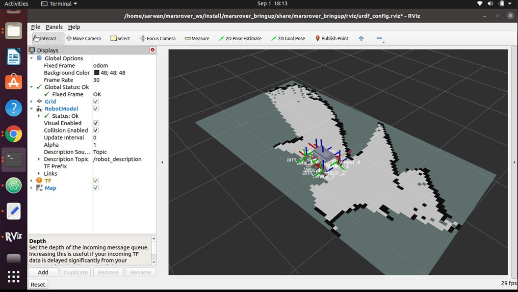
Recorded in RViz. Teleop commands go through the Ackermann controller node. The odometry node moves the model
in the odom frame, and the steering joints follow the controller output.
Controller board
OpenCR 1.0
Servos
10 × Dynamixel XL430 (4 in position mode, 6 in velocity mode)
Onboard computer
Jetson AGX Xavier
Depth camera
Intel RealSense D435
Tracking camera
Intel RealSense T265
Battery
5800 mAh LiPo
Remote control
Taranis X9 Lite
Languages
C++, Python
Libraries
Dynamixel2Arduino
Mapping
SLAM Toolbox, RTAB-Map
Overview
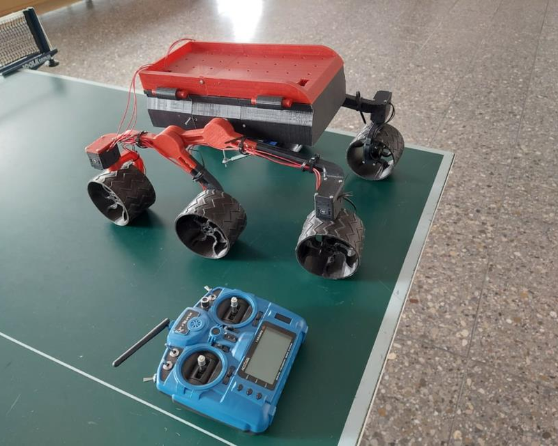
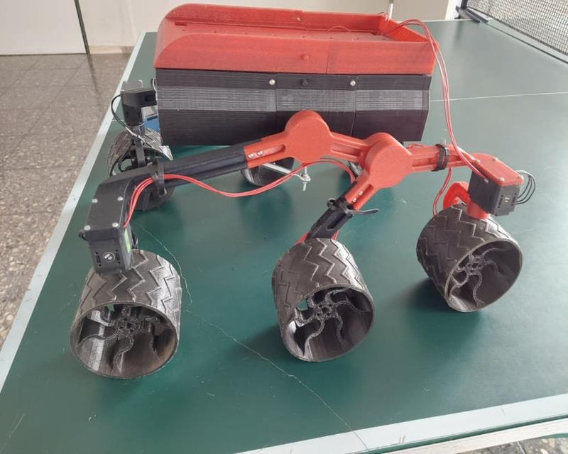
I took over a 3D-printed, six-wheel rover modelled on NASA's Mars rovers. An earlier student group had
designed it. Over two university R&D modules in 2021, I assembled it, made it drive and wrote
its control system twice.
Phase 1, Arduino. Ackermann steering and an electronic differential on the OpenCR board, driven by a hobby RC transmitter.
Phase 2, ROS 2. The same kinematics as a ROS 2 node on a Jetson AGX Xavier. micro-ROS links it to the servos. Wheel odometry, a URDF model, keyboard and gamepad teleop, and 2D mapping with a depth camera complete the stack.
Phase 1: Ackermann steering, worked simply
Ackermann steering solves the difference of angles between
steering wheels during vehicle turning. This difference is caused by the fact that each wheel
follows a different radius, so that the inside wheel has to be tilted a little more than the outside
wheel. This principle radically reduces tire slippage (that is important especially at higher
speeds). The Ackerman concept is to have all wheels rolling around a common point called
Instantaneous center (ICC) during a turn. This can greatly improve cornering ability and
performance. The correct angles are dependent on the wheelbase of the vehicle and the angle
of turn.
Left turn with a 30° virtual steering angle, drawn to scale. R is measured from the ICR to the rover centre.
T is half the track (0.154 m) and L is the front-to-middle axle distance (0.2 m).
The whole controller comes down to three lines. The driver's remote controller gives a virtual steering angle δ for an imaginary wheel in the middle of the front axle:
R = L / tan(δ)
δ_in = atan( L / (R − T) ) δ_out = atan( L / (R + T) )
ω = v / R v_in = ω · (R − T) v_out = ω · (R + T)
The first line places the ICR. The second gives each steered wheel the angle that points it around the
ICR, so the inner wheel always steers more. The third is a software differential. The whole rover
turns at one angular velocity ω, so wheels on the outside of the curve must roll faster than wheels on the inside.
Phase 1: Dynamixel and Arduino control
Phase 1 signal path. All 10 servos sit on daisy-chained TTL buses, one per side of the rover.
Two servo modes. The 4 steering servos run in position mode with the range limited to 135 - 225° (180° is straight ahead). The 6 drive servos run in velocity mode, so the code can command wheel rpm directly with no PWM mapping.
Why not multi-turn mode for steering. A Dynamixel can make a full rotation to re-home after a mode change or power reset. On a steering joint, that would tear out the wiring. Using single-turn position mode with hard limits rules this out.
Setting PID gains for smooth motion. As an inital step, I tested PID gains and motion profiles in Dynamixel Wizard 2.0. The startup code then sets a profile velocity on the steering servos and a profile acceleration on the drive servos, so the servos ramp to each new goal instead of jumping.
One wire for 8 channels. PWM output would need one wire and one interrupt pin per channel. The receiver's PPM output carries all channels on a single wire, decoded by one interrupt.
Failsafe on signal loss. The transmitter failsafe sets the throttle channel to its centre value (1500 µs), and the control loop treats this as stop.
Drive modes. A 1485 - 1515 µs dead band on each RC lever selects between forward, reverse, Ackermann turns forward and reverse, steering on the spot, and spin in place. For spinning, a switch sets the corner wheels tangent to a circle and runs all six wheels in the same direction.
The PPM decoder
The interrupt timestamps every pulse with micros(). The gap between two pulses is one channel value, about 1000–2000 µs.
A gap longer than 3000 µs can only be the sync pause, so the decoder restarts at channel 1.
// Stores the pulse position timers
void my_ISR() {
    byte state_now = digitalRead(my_pin);
    if (state_now == my_state) {
        timers[pulse] = micros();
        if (pulse > 0) {
            getChannelValue(pulse);
        } else pulse++;
    }
}

// Calculates the channel values
void getChannelValue(byte pointer) {
    channels[pointer -1] = timers[pointer] - timers[pointer -1];
    if (channels[pointer -1] > 3000) {        // sync gap: new frame
        timers[0] = timers[pointer];
        pulse = 1;
    } else pulse++;
}
From PPM.cpp, a small library I wrote as a .hpp/.cpp pair.
RC to wheel angle
The three formulas above, as they run on the board. The RC output is mapped to 0–30° of virtual steering, and the result maps onto the servo's absolute angle.
From LeftTurn() in Rover.ino. RightTurn() mirrors it.
Phase 2: the same control in ROS 2
In phase 2 the rover gets an onboard computer (Jetson AGX Xavier) and depth cameras, and the control moves into ROS 2.
The key change is the input. Instead of a RC angle, the controller accepts a standard
geometry_msgs/Twist (forward speed v, turn rate ω). A Nav2 navigation stack sends the same message, so
the controller is ready for autonomous driving later.
Phase 2 node graph. The Ackermann math from phase 1 now lives in one ROS 2 node. The OpenCR only translates messages to servo commands and reports encoder ticks.
From Twist to wheel commands
R = v / ω (clipped to 0.4 m … 11 m; larger R is treated as straight)
then the same δ_in, δ_out and wheel speeds as in phase 1
Better corner wheel speeds. The Arduino version gave all wheels on one side the same speed. The ROS node uses each wheel's real distance from the ICR. Corner wheels sit further out than middle wheels, so they get ω · √((R ± T)² + L²).
Speed capped in tight turns. In a turn the outer wheels must run faster than the rover centre. The node lowers the centre speed so the outer wheels never exceed what the servo can deliver.
Units at the boundary. The node publishes wheel speeds in rad/s and steering angles in radians. The micro-ROS sketch converts them for the servos (× 9.55 for rpm, × 57.3 for degrees).
From control_logic.py. The structure follows NASA JPL's Open Source Rover kinematics code,
adapted to this rover's dimensions, servos and ROS 2.
Wheel odometry
The OpenCR reads the encoder position of the two middle wheels and publishes the raw ticks every 100 ms.
The odometry node turns tick differences into wheel speeds and then into rover motion. This is the
standard differential-drive model, which fits because the middle wheels never steer.
v_L, v_R = (Δticks * 2π / 4096) / Δt * r
v = (v_R + v_L) / 2 ω = (v_R - v_L) / track
x += v·cos θ·Δt y += v·sin θ·Δt θ += ω·Δt
The node publishes the pose as nav_msgs/Odometry and as the TF odom → base_footprint.
It also publishes joint_states for the wheels and steering joints, so the URDF model in RViz moves like the rover.
Rest of the stack
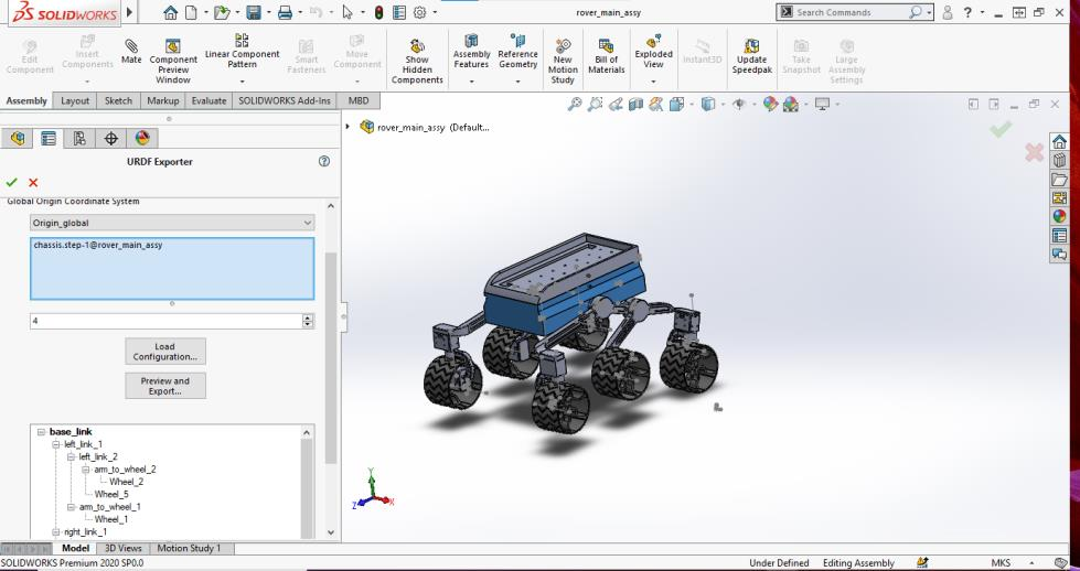
URDF exported from the SolidWorks assembly with the sw_urdf exporter. I added base_footprint, camera and T265 links by hand.
Teleop with a keyboard node or an Xbox controller through joy. A mapping node constrains the axes to the rover's speed limits.
2D mapping. The D435 point cloud goes through pointcloud_to_laserscan, and SLAM Toolbox builds an occupancy map from the scan and the wheel odometry.
Networking. The Jetson and the laptop share a ROS_DOMAIN_ID over Wi-Fi, so RViz runs on the laptop while the nodes run on the rover.
Building the URDF in SolidWorks. The exporter turns the assembly into a link tree, from base_link through the rocker and bogie links to each wheel.A 2D occupancy map from SLAM Toolbox in RViz, with the rover model and its TF frames at the current pose.